Introduction
Autonomous robots having a non-holonomic kinematics motion model results in a non-linear mapping between the control inputs and the states. Trajectory optimization problems with such motion models takes the form of a challenging non-linear programming problem (NLP).
Model Predictive Controls are good at solving this non-linear trajectory optimization problem. Here we use the model of the vehicle to predict the controls of the vehicle upto \(T\) timesteps into the future. The control signals are usually obtained by minimizing an objective function while satisfying a set of constraints.
Usually techniques like sequential quadratic programming (SQP) are used to obtain a locally optimal solution. But it requires that we convexify the non-linear and non-convex trajectory optimization problem. We do this by linearizing the system model incorporating the path constraints including collision avoidance constraints by introducing them as penalty terms in the objective functions. These linear approximations may often lead to infeasible solutions resulting in collisions with the obstacles.
The paper “An nmpc approach using convex inner approximations for online motion planning with guaranteed collision avoidance” (CIAO) proposed the use of convex inner approximations to plan the trajectories. The Convex Inner Approximation method finds kinodynamically feasible trajectories that guarantees collision avoidance. It also finds the trajectories in fewer iterations and as a result is much faster.
For my Google Summer of Code 2022 project with the Robocomp organization, I proposed and implemented the CIAO paper in their optimizer component for an indoor robot navigation scenario. The final result is a robot that is able to navigate in complex narrow corridors while avoiding static and dynamic obstacles.
Contributions
Phase 1
- Added acceleration constraints. [Pull Request #3]
- Added euclidean distance obstacle avoidance constraints. [Pull Request #4]
- Added a feature such that if the target is behind the robot, the robot will first rotate on spot and then start moving towards the obstacle. [Pull Request #5]
Phase 2
- Added a feature that will move the target to the nearest free cell if it is given inside an obstacle. [Pull Request #377]
- Added a feature that allows the robot to navigate through narrow corridors which was previously not possible because of overconstrained representation of the obstacles in the occupancy grid map. [Pull Request #379]
- Implementation of the CIAO paper with automatic weights tuning. [Pull Request#9]
Formulation
The state configuration of the vehicle is represented as the vector \(\begin{bmatrix}x_t, y_t, \theta_t\end{bmatrix}^T\) where \(x_t\) is the \(x\) coordinate of the agent at timestep \(t\), \(y_t\) is the \(y\) coordinate of the agent at timestep \(t\) and \(\theta_t\) is the orientation of the agent at timestep \(t\).
We use the unicycle kinematics vehicle model to represent the vehicle. The configuration transition equation of the unicycle model is given as:
\[\begin{align} \dot{x} &= v \cos \theta \\ \dot{y} &= v \sin \theta \\ \dot{\theta} &= \omega \end{align}\]Here we formulate the path optimization problem with the variables as linear velocities \(v_{t_i}\) and angualar velocities \(\omega _{t_i}\) over the time interval \([t_i, t_{i+n}]\). The cost funtion is written as:
\[\begin{align} \displaystyle{\min_{v,w} (x_N(\textbf{v},\textbf{w}) - x_g)^2 + (y_N(\textbf{v},\textbf{w}) - y_g)^2 + (\theta_N(\textbf{v},\textbf{w}) - \theta_g)^2} \end{align}\]Here \(x_N\) is a function that takes the vector of velocities \(\textbf{v}\) and angular velocities \(\textbf{w}\) as input and uses the unicycle kinematics model of the vehicle to give the \(x\) coordinate of the vehicle at the \(N\)-th timestep. The function \(y_N\) and \(\theta_N\) gives the \(y\) and \(\theta\) of the vehicle in the \(N\)-th timestep in the same manner. The above cost function ensures that the \(N\)-th position of the vehicle is the closest to the goal configuration of the vehicle.
Since the autonomous vehicles have a maximum and minimum velocity, angular velocity and acceleration and angular acceleration bounds, we add them as bound constraints to the cost function:
\[\begin{align} v_{min} \leq \mathbf{v}\leq v_{max} \\ \omega_{min} \leq \boldsymbol{\omega} \leq \omega_{max} \\ a_{min} \leq \mathbf{a} \leq a_{max} \\ \alpha_{min} \leq \boldsymbol{\alpha} \leq \alpha_{max} \end{align}\]Usually the obstacles and the agent are represented as circles. The obstacle avoidance constraints are given as:
\[\begin{align} d(A_{pos_t}, O^i_{pos_t}) \geq r_a + r^i_o \end{align}\]Here \(A_{pos_t}\) is the position of the agent at timestep \(t\) such that \(1 \leq t \leq T\) and \(O^i_{pos_t}\) is position the obstacle \(i\) at timestep \(t\) such that \(1 \leq i \leq N\) and \(1 \leq t \leq T\) . \(d(A_{pos_t}, O^i_{pos_t})\) is the euclidean distance between the agent and obstacle \(i\) at timestep \(t\). \(r_a\) is the radius of the agent and \(r_o\) is the radius of the obstacle.
Representing obstacle avoidance constraints as Convex Inner Approximation
The obstacle avoidance constraint mentioned above is non-convex and non-linear and hence is ill-suited for rapid optimization. To solve for this we take the Convex Inner Approximation of the constraints that is based on the notion of free balls.
Let \(\mathscr{O}\) be the occupied set and \(\underline{d} > 0\) be the minimum distance, then the free set \(\mathscr{A}\) is defined as \(\mathscr{A} = \{a \in \mathscr{W}: \Vert a - o \Vert _2 \geq \underline{d}, \forall o \in \mathscr{O} \}\)
Here \(\mathscr{W}\) is the robot’s workspace.
The above definition implies that the free set \(\mathscr{A}\) and the occupied set \(\mathscr{O}\) are disjoint.
An obstacle avoidance constraint can now be formulated by making sure that the robot’s position always lies within an n-dimensional ball formed around \(c \in \mathscr{A}\).
For an arbitrary free point \(c \in \mathscr{A}\) we define the free ball as
\[\mathscr{A}_c := \{ p \in W : \Vert p - c \Vert _2 \leq d_\mathscr{O}(c) - \underline{d} \}\]The free ball is a convex subset of the free set \(\mathscr{A}\).
The collision avoidance constraint \(\Vert p - c \Vert _2 \leq d_\mathscr{O}(c) - \underline{d}\) is not differentiable so we square both sides to make it differentiable. The new constraint looks like this: \(\Vert p - c \Vert _2 ^2 \leq (d_\mathscr{O}(c) - \underline{d})^2\). \(c\) represents the free-ball center points and we need to find them first before solving for the trajectory.
CIAO Iteration
Given an initial guess \(w\) where \(w = \begin{bmatrix} x_0^T, u_0^T, \dots, x_N^T, u_N^T \end{bmatrix}^T\) is a vector of optimization variables that contains the stacked controls and states for all \(N\) steps in the planning horizon, we find the first set of the center-point vector \(C\) as
\[C \leftarrow (c_k \in S_p . x_k \text{ for }k = 0, 1, \dots, N)\]Here \(S_p\) is the selector matrix and we are getiing the \(x_k\) values from the initial guess.
The free balls resulting from these center-points might be very small and restrictive especially if the initial guess is too close to the obstacles. To solve this issue we maximize the free balls by solving the optimization problem for each center-point \(c\) such that we get the optimal centerpoint \(c^* = \eta .g + c\)
\[\begin{align} \displaystyle{\max_{\eta \geq 0} \eta \text{ s.t. } d_\mathscr{O}(\eta . g + c) = \eta + d_\mathscr{O}(c) } \end{align}\]Here \(\eta\) is the step size and \(g\) is the search direction with \(\Vert g \Vert_2 = 1\)
Once we get the center-point vectors we can solve the trajectory optimization problem as
\[\begin{align} \displaystyle{\min_{\textbf{w},\textbf{s}} J( \textbf{w}) + \sum_{k=0} ^N \mu_k . s_k } &\\ s.t. \text{ } \Vert p - c \Vert _2 ^2 &\leq (d_\mathscr{O}(c) - \underline{d})^2 + s_k \end{align}\]Advantages
In traditional euclidean distance obstacle avoidance constraints, we estimate the robot and the obstacles as circles and for every timesteps we make sure that the distance between the robot and the obstacles are a minimum of the sum of their radius. Therefore given a set of \(N\) obstacles, and if we are planning for \(T\) timesteps, for every timestep we will have \(N\) obstacle avoidance constraints and in total we will have \(N \times T\) constraints. These are too many constraints and if the number of obstacles increases then the computation can’t be done in real-time.
Using CIAO, we will have only \(1\) obstacle constraint for each timestep. And for \(T\) timestep, we will have \(T\) obstacle avoidance constraints. This decreases the number of obstacle avoidance constraints significantly and therefore also improves computation times and as a result is a lot faster.
Simplified explanation of the CIAO algorithm
The robot’s pose is given by the vector \(\begin{bmatrix}x \\ y \\ z \end{bmatrix}\). If we are planning for \(T\) timesteps into the future, we have \(T\) such poses.
Let us assume that we know the positions of all the obstacles.
Given a set of \(T\) poses of the robot which we will call initial guess, we will first modify these poses such that they are at a distance from the nearest obstacle from which we can draw the biggest circle possible with the initial guesses as centers of the circle. We will update the previous initial guesses to these new poses and we will also keep a record of the radius of the circles.
Now we will compute another set of new poses which will be the robot’s pose in each timestep \(t\) where \(0 \leq t \leq T\). These poses will try to be as close to the center of the circle as possible and will always try to be inside the radius of the circles. These poses will also be calculated considering various constraints of the robot like it’s maximum velocity limit and maximum acceleration bounds.
As long as the robot stays inside the circles, it will avoid the obstacles.
Environment
run_beta
A simple environment with one movable block. Useful for testing if an obstacle avoidance algorithm is working by moving the block towards the robot and seeing if the planned trajectory avoids it.
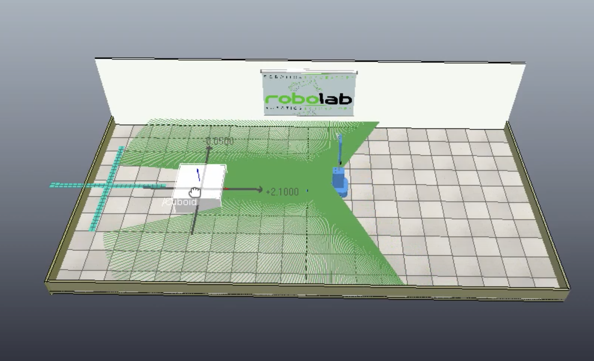
Fig. 1. run_beta environment
run_beta_bill
The run_beta environment with two static obstacles and one static human (Bill). Useful for testing obstacle avoidance in lightly cluttered environments.
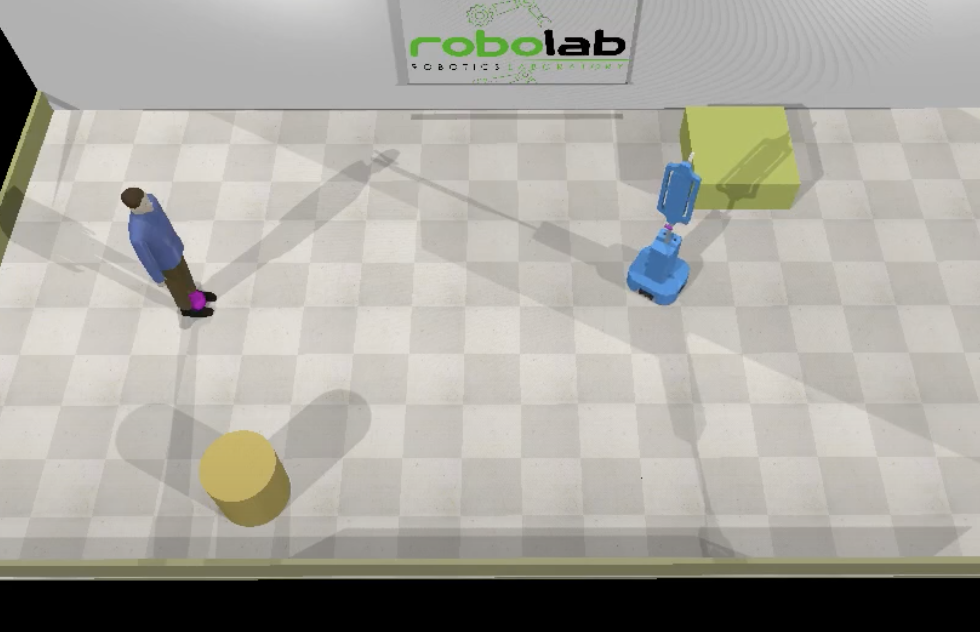
Fig. 2. run_beta_bill environment
run_beta_bill_walking
An environment with two static obstacles that also create a narrow corridor. There is also a walking human (Bill). This is a good environment to test if our algorithm is working with dynamic obstacles in cluttered scenes.
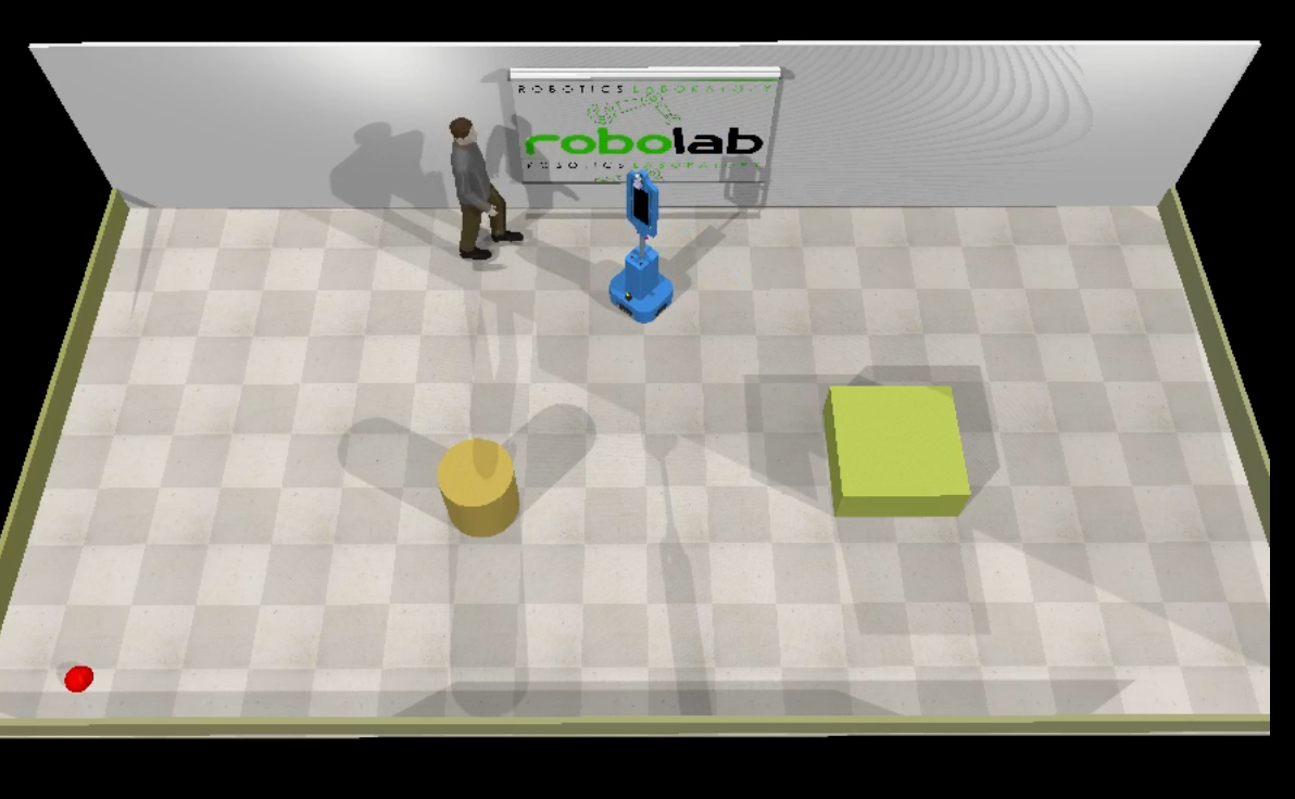
Fig. 3. run_beta_bill_walking environment
run_beta_infirmary
A complex environment with 6 rooms. No dynamic obstalces but there are a lot of narrow doorways. A good environment to check if the obstacle avoidance constraints are working and allows the robot to pass through the narrow doorways.
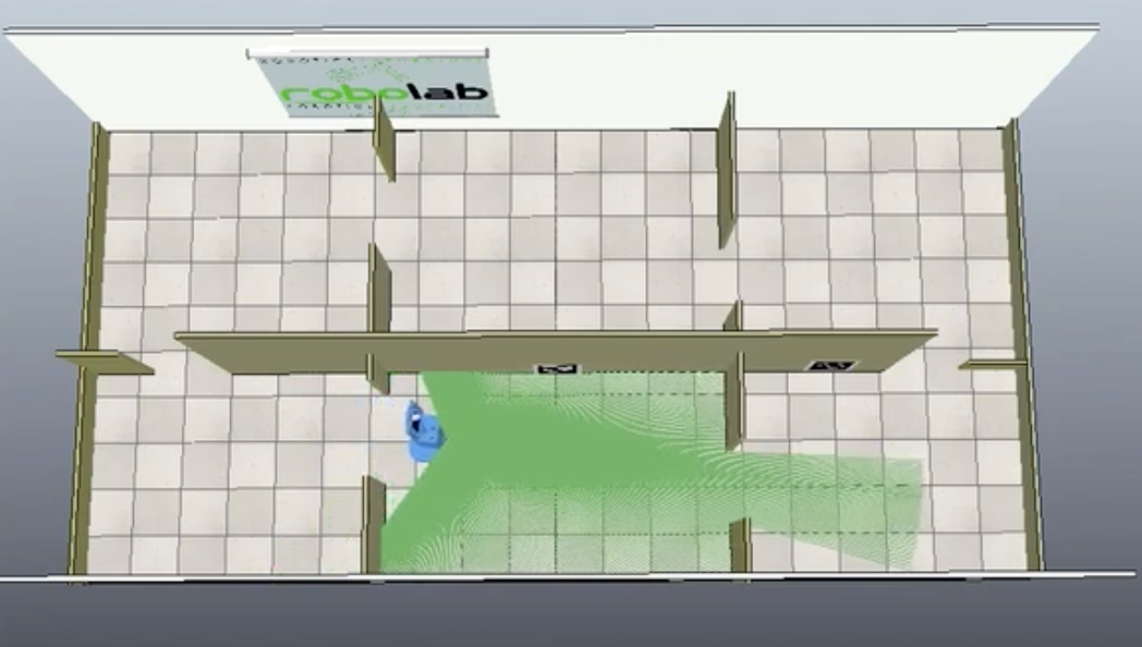
Fig. 4. run_beta_infirmary environment
run_beta_infirmary_with_bill
The run_beta_infirmary environment with a walking human (Bill) to simulate a moving human. Good for testing obstacle avoidance algorithm in complex environment.
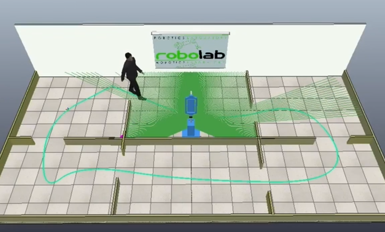
Fig. 5. run_beta_infirmary_with_bill environment
Results
Phase 1
Vid. 1.1. Video demonstrating obstacle avoidance using euclidean distance obstacle avoidance constraints.
Vid. 1.2. Video demonstrating obstacle avoidance using euclidean distance obstacle avoidance constraints to avoid a walking human (Bill).
Phase 2
Vid. 2.1. Video demonstrating that the agent won’t crash to the obstacle if the target is given inside the obstacle.
Vid. 2.2. Video showing the robot’s ability to pass through narrow corridors using euclidean distance obstacle avoidance constraints.
Vid. 2.3. CIAO implementation with automatic weight tuning in run_beta_infirmary environment.
Vid. 2.4. CIAO implementation with automatic weight tuning in run_beta_infirmary_with_bill environment.
Conclusion
While the free balls algorithm works really well in complex environment, there are much to be explored on how we can speed up the computation time to compute the trajectories more efficiently. One approach would be to come up with better ways to initialize the optimizer. Another approach can be to make the trajectory optimization formulation differentiable. Having a differentiable formulation will enable us to integrate the trajectory computation with the perception system in an end to end manner.