- Inverse matrix
- Vector spaces
- Subspaces
- Span
- Basis
- Four fundamental subspaces
- Solving \(Ax=0\) and special solutions
- Orthogonality
- Projections
- Orthonormal vectors
- Determinant of a matrix
- Eigen values and eigen vectors
- Symmetric matrices
- Positive definite marices
- Similar Matrices
- Singular value decomposition
Inverse matrix
If two matrices \(A\) and \(B\) are multiplicable, then their product will give a third matrix \(C\). This means that the transformation matrix \(A\) transforms the matrix \(B\) to the matrix \(C\). Now if we want to go back from the matrix \(C\) to matrix \(B\), we will be multiplying the inverse of the transformation matrix \(A\) represented as \(A^{-1}\) to the transformed matrix \(C\). To understand intuitively, whatever the transformation matrix does, the inverse matrix undoes. However not all transformation matrices have an inverse. When a transformation matrix have dependent rows or dependent columns, then that transformation matrix does not have an inverse. Also only square matrices can have an inverse.
The inverse of the product of two matrices is:
\[(AB)^{-1}=B^{-1}A^{-1}\]We can use the Gauss-Jordan method to find the inverse of a matrix.
Suppose we have a matrix \(A=\begin{bmatrix}1 & 3\\ 2 & 7\end{bmatrix}\). Let \(A^{-1}=\begin{bmatrix}a & b\\ c & d\end{bmatrix}\).
We know that \(AA^{-1}=I\). Therefore we can say
\[A=\begin{bmatrix}1 & 3\\ 2 & 7\end{bmatrix}\begin{bmatrix}a & b\\ c & d\end{bmatrix}=\begin{bmatrix}1 & 0\\ 0 & 1\end{bmatrix}\]To solve this, we can write in the form
\[\left[ \begin{array}{cc|cc} 1 & 3 & 1 & 0 \\ 2 & 7 & 0 & 1 \end{array} \right]\]This is called an augmented matrix. Here the left-hand side of \(\mid\) represents matrix \(A\) and the right-hand side of \(\mid\) represents the identity matrix \(I\). To find the pivots on the side representing \(A\) we use elimination and get
\[\left[ \begin{array}{cc|cc} 1 & 3 & 1 & 0 \\ 0 & 1 & -2 & 1 \end{array} \right]\]Since the left-hand side is in upper triangular form, we now use elimination upwards to get
\[\left[ \begin{array}{cc|cc} 1 & 0 & 7 & -3 \\ 0 & 1 & -2 & 1 \end{array} \right]\]If we write the operations that we performed in the form of a transformation matrix \(E\), then we can write \(E[A\mid I]=[I\mid E]\). Since \(EA\) produces \(I\), therefore we can say \(E\) is \(A^{-1}\) and thus we solve for \(A^{-1}\).
Vector spaces
In two dimensional vectors, the vectors have two components that represents the \(x\) coordinates and \(y\) coordinates of the two-dimensional plane. This two-dimensional plane is called a vector space. If we pick any two vectors from this two-dimensional plane, their linear combination will always lie in the plane. As a rule of thumb, if we take any number of vectors from a vector space, their linear combination will always lie in that vector space. Some other examples of vector spaces are the three-dimensional space, four-dimensional space and so on.
Subspaces
From the two-dimensional space, if we pick a line that passes through the \(\begin{bmatrix}0 & 0\end{bmatrix}^T\) vector, we will notice that this line acts like a vector space as-well. If we pick any vectors on this line we will see that their linear combination will always lie on this line. This line is called the subspace of the two-dimensional vector space. A subspace is a vector space contained inside another vector space and must always contain the zero vector. A vector space can have multiple subspaces.
If we are given two subspaces \(P\) and \(L\). Then their union \(P \cup L\) is not a subsapace but their intersection \(P \cap L\) is a subspace.
Some examples of the possible subspaces of the three-dimensional vector space are:
-
Any line through the zero vector \(\begin{bmatrix}0 & 0 & 0\end{bmatrix}^T\).
-
The whole three-dimensional vector space is also a subspace.
-
Any plane through the zero vector \(\begin{bmatrix}0 & 0 & 0\end{bmatrix}^T\).
-
The zero vector \(\begin{bmatrix}0 & 0 & 0\end{bmatrix}^T\)
Span
We are given two vectors \(\begin{bmatrix}0 & 1\end{bmatrix}^T\) and \(\begin{bmatrix}1 & 0\end{bmatrix}^T\). These two vectors lie on the two-dimensional vector space. If we pick any vector from this space, it will be a linear combination of these two vectors. That is why these two vectors are said to span the space.
Vectors \(\boldsymbol{v_1}, \boldsymbol{v_2}, \dots \boldsymbol{v_n}\) are said to span a space when the space consists of all linear combinations of those vectors. If vectors \(\boldsymbol{v_1}, \boldsymbol{v_2}, \dots \boldsymbol{v_n}\) span a space \(S\), then \(S\) is the smallest space containing those vectors.
Basis
If we are given a sequence of vectors \(\boldsymbol{v_1}, \boldsymbol{v_2}, \dots \boldsymbol{v_n}\) such that they are independent and they span a vector space, then these vectors are said to form the basis for that vector space.
Given a vector space, every basis of that space has the same number of vectors. That number is called the dimension of that space.
There are exactly \(n\) vectors in every basis for the n-dimensional space.
Four fundamental subspaces
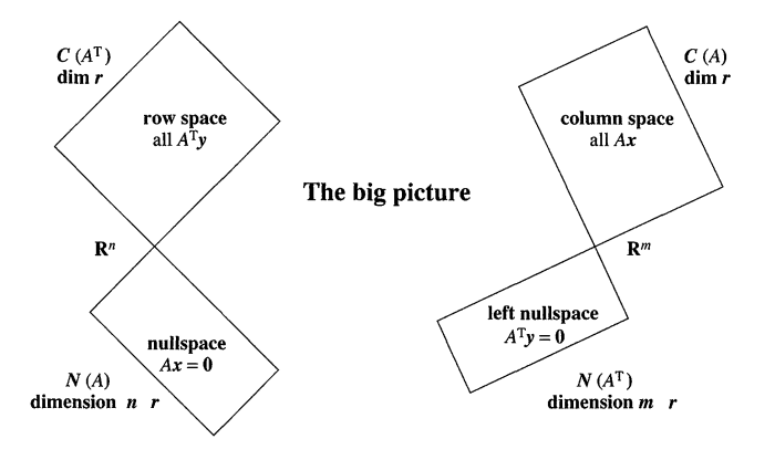
Fig. 1. The four fundamental subspaces. (Image source: Sec 3.6 Strang, Gilbert. Introduction to Linear Algebra, 2009.)
Column Space
The column space of a matrix is all the linear combinations of the columns of the matrix.
Suppose we have a matrix
\[A=\begin{bmatrix} 1 & 3\\ 2 & 3\\ 4 & 1\end{bmatrix}\]The column space of A will contain all the linear combinations of the vectors
\[\begin{bmatrix}1 \\ 2 \\ 4\end{bmatrix}\]and
\[\begin{bmatrix}3 \\ 3 \\ 1\end{bmatrix}\]To understand the column space in terms of the equation \(A\boldsymbol{x}=\boldsymbol{b}\), \(\boldsymbol{b}\) is the linear combination of the columns of the matrix \(A\). Therefore, \(\boldsymbol{b}\) has to be in the column space produced by \(A\) for the system to have a solution \(\boldsymbol{x}\) else \(A\boldsymbol{x}=\boldsymbol{b}\) is unsolvable. The column space of a matrix \(A\) is represented as \(C(A)\). For a matrix \(A\) with \(m\) rows and \(n\) columns, the column space of \(A\) will be a subspace of the vector space \(R^m\).
Null Space
The null space of a matrix \(A\) contains all the solution vectors \(\boldsymbol{x}\) to the equation \(A\boldsymbol{x}=0\). \(A\boldsymbol{x}\) is the linear combination of the column vectors of \(A\). When the null space of \(A\) contains only the zero vector, then the column vectors of \(A\) are said to be independent. For a matrix \(A\) with \(m\) rows and \(n\) columns, the null space of \(A\) will be a subspace of the vector space \(R^n\).
Row Space
The row space of a matrix is all the linear combinations of the rows of the matrix.
For the matrix
\[A=\begin{bmatrix} 1 & 3\\ 2 & 3\\ 4 & 1\end{bmatrix}\]the row space will contain all the linear combinations of the rows \(\begin{bmatrix} 1 & 3\end{bmatrix}\), \(\begin{bmatrix} 2 & 3\end{bmatrix}\) and \(\begin{bmatrix} 4 & 1\end{bmatrix}\) of the matrix. The row space of a matrix \(A\) is represented as \(C(A^T)\) because the rows of the matrix \(A\) will become the columns of the matrix \(A^T\). Therefore we can say that the row space of \(A\) is the column space of \(A^T\). For a matrix \(A\) with \(m\) rows and \(n\) columns, the row space of \(A\) will be a subspace of the vector space \(R^n\).
Left Null Space
This is also called the null space of \(A^T\). The null space of the matrix \(A^T\) contains all the solutions \(\boldsymbol{y}\) to the equation \(A^T\boldsymbol{y}=0\). \(A^T\boldsymbol{y}\) is the linear combination of the row vectors of \(A\) or the column vectors of \(A^T\). For a matrix \(A\) with \(m\) rows and \(n\) columns, \(A^T\) will have \(n\) rows and \(m\) columns. The null space of \(A^T\) will be a subspace of the vector space \(R^m\).
Solving \(Ax=0\) and special solutions
Let
\[A=\begin{bmatrix} 1 & 2 & 2 & 2\\ 2 & 4 & 6 & 8\\ 3 & 6 & 8 & 10\end{bmatrix}\]If we reduce \(A\) to it’s echelon form \(U\), we will have
\[U=\begin{bmatrix} 1 & 2 & 2 & 2\\ 0 & 0 & 2 & 4\\ 0 & 0 & 0 & 0\end{bmatrix}\]Here the first pivot is the first element of the first column i.e. \(1\). We don’t find a pivot in the second column, so our next pivot is the \(2\) in the third column of the second row. The first and the third columns are called the pivot columns as they contain the pivots, and the variables which form the pivot elements in these pivot columns are called the pivot variables. The remaining columns are called free columns.
In our matrix \(A\), columns \(1\) and \(3\) are the pivot columns while columns \(2\) and \(4\) are the free columns. Therefore in our solution vector \(x=\begin{bmatrix} x_1 & x_2 & x_3 & x_4 \end{bmatrix}^T\), we can assign any value to \(x_2\) and \(x_4\) as these variables multiply with the free columns. These variables are called free variables. Suppose we assign \(x_2=1\) and \(x_4=0\).
Then \(2x_3+4x_4=0 \implies x_3=0\)
and \(x_1+2x_2+2x_3+2x_4=0 \implies x_1=-2\)
Thus one of the solution vectors is \(x=\begin{bmatrix} -2 & 1 & 0 & 0\end{bmatrix}^T\). The solution vector means that \(-2\) times the first column added with the second column will give us the zero vector. Therefore any multiple of the solution vector \(x\) will also give the zero vector and thus a solution.
Similarly if we assign \(x_2=0\) and \(x_4=1\). Then we get the solution vector as: \(x=\begin{bmatrix} 2 & 0 & -2 & 1\end{bmatrix}^T\). This solution vector means that \(2\) times the first column added with \(-2\) times the third column added with the fourth column will give us the zero vector. Also any multiple of this solution vector will also give us a zero vector and thus a solution. The two solution vectors that we got are called special solutions. The solution \(x\) is the collection of all the linear combinations of these special solution vectors.
The number of free columns in the matrix is the rank of the matrix subtracted from the number of columns of the matrix (\(n-r\)). The number of special solutions is equal to the number of free columns of the matrix. The solution \(x\) for the equation \(Ax=0\) is the collection of the linear combination of all the special solutions of the matrix. These solutions for the equation \(Ax=0\) form the null space of the matrix \(A\).
Orthogonality
Two vectors \(\boldsymbol{x}\) and \(\boldsymbol{y}\) are said to be orthogonal if \(\boldsymbol{x}^T\boldsymbol{y}=0\). Orthogonal means perpendicular, i.e. the vectors \(\boldsymbol{x}\) and \(\boldsymbol{y}\) are perpendicular to each other. All vectors are orthogonal to the zero vector.
Two subspaces \(S\) and \(T\) are said to be orthogonal to each other if all the vectors in subspace \(S\) are orthogonal to all the vectors in subspace \(T\). For example, the row space of a matrix is orthogonal to the nullspace of that matrix and the column space of that matrix is orthogonal to the left null space of that matrix.
Projections
The equation \(A\boldsymbol{x}=\boldsymbol{b}\) will have a solution only when \(\boldsymbol{b}\) lies on the column space of \(A\). However sometimes, due to measurement error, \(\boldsymbol{b}\) might not lie on the column space of \(A\) and therefore \(A\boldsymbol{x}=\boldsymbol{b}\) will have no solution. So to find the best possible solution, we project vector \(\boldsymbol{b}\) onto a vector \(\boldsymbol{p}\). The vector \(\boldsymbol{p}\) lies on the column space of \(A\). We then solve for \(A\boldsymbol{\hat{x}}=\boldsymbol{p}\) where \(\boldsymbol{\hat{x}}\) is the best possible solution for \(A\boldsymbol{x}=\boldsymbol{b}\).
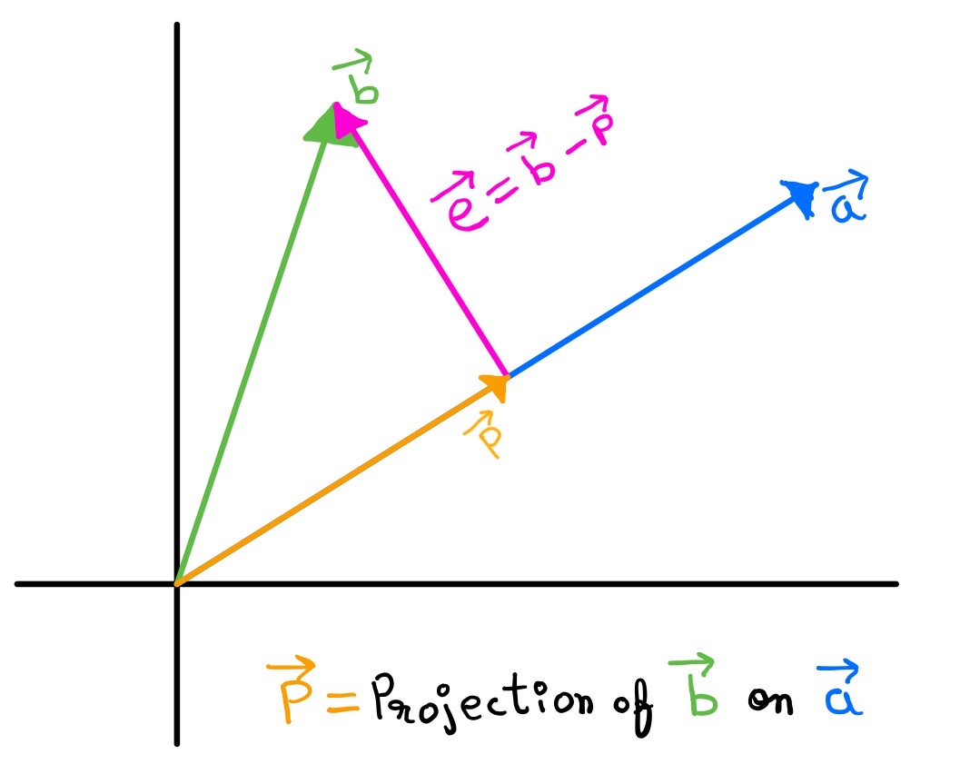
Fig. 2. Projection of vector \(\boldsymbol{b}\) on vector \(\boldsymbol{a}\).
If we have a vector \(\boldsymbol{b}\) and the line determined by a vector \(\boldsymbol{a}\), we do the projection of \(\boldsymbol{b}\) on line \(\boldsymbol{a}\) to find the vector \(\boldsymbol{p}\).
Here, the vector \(\boldsymbol{p}\) is a scalar multiple of vector \(\boldsymbol{a}\).
\[\boldsymbol{p}=x\boldsymbol{a}\]Now from the figure we can see that the vector \(\boldsymbol{a}\) is orthogonal to the vector \(\boldsymbol{e}\). Therefore
\[\boldsymbol{a^T}\boldsymbol{e}=0\] \[\implies \boldsymbol{a^T}(\boldsymbol{b}-\boldsymbol{p})=0\] \[\implies \boldsymbol{a^T}(\boldsymbol{b}-x\boldsymbol{a})=0\] \[\implies x\boldsymbol{a^T}\boldsymbol{a}=\boldsymbol{a^T}\boldsymbol{b}\] \[\implies x=\dfrac{\boldsymbol{a^T}\boldsymbol{b}}{\boldsymbol{a^T}\boldsymbol{a}}\]Therefore we can write
\[\boldsymbol{p}=\boldsymbol{a}x \implies \boldsymbol{p}=\dfrac{\boldsymbol{a}\boldsymbol{a^T}\boldsymbol{b}}{\boldsymbol{a^T}\boldsymbol{a}}\]Projection matrix
Now we want to write this projection in terms of a projection matrix \(P\) such that \(\boldsymbol{p}=P\boldsymbol{b}\).
Therefore we can write the projection matrix \(P\) as
\[P=\dfrac{\boldsymbol{a}\boldsymbol{a^T}}{\boldsymbol{a^T}\boldsymbol{a}}\]The column space of the matrix \(P\) is spanned by the line \(\boldsymbol{a}\) because for any \(\boldsymbol{b}\), \(P\boldsymbol{b}\) lies on \(\boldsymbol{a}\) which means \(\boldsymbol{a}\) is the linear combination of the columns of the matrix \(P\).
The projection matrix \(P\) is a symmetric matrix which means \(P^2\boldsymbol{b}=P\boldsymbol{b}\) because the projection of the vector already on the line \(\boldsymbol{a}\) will be the same vector only.
Projection matrix in high dimensional spaces
Here we will see what the projection matrix will be like in a higher dimensional space like \(R^3\).
Suppose in \(R^3\), we want to project a vector \(\boldsymbol{b}\) onto a vector \(\boldsymbol{p}\) that lies on a plane. If \(\boldsymbol{a_1}\) and \(\boldsymbol{a_2}\) form the basis for the plane, then the plane is the columnspace of the matrix \(\begin{bmatrix}a_1 & a_2\end{bmatrix}\). For the projection vector of \(\boldsymbol{b}\), \(\boldsymbol{p}\) must be a linear combination of \(\boldsymbol{a_1}\) and \(\boldsymbol{a_2}\) for it to lie on the plane. Therefore we can write
\[\hat{x_1}\boldsymbol{a_1}+\hat{x_2}\boldsymbol{a_2}=\boldsymbol{p}\] \[\implies \begin{bmatrix} \boldsymbol{a_1} & \boldsymbol{a_2}\end{bmatrix}\begin{bmatrix}\hat{x_1}\\ \hat{x_2}\end{bmatrix}=\boldsymbol{p}\] \[\implies A\boldsymbol{\hat{x}}=\boldsymbol{p}\]If \(\boldsymbol{e}=\boldsymbol{b}-\boldsymbol{p}\) and \(\boldsymbol{e}\) is orthogonal to the plane, then \(\boldsymbol{e}\) is orthogonal to any vector on the plane. Therefore
\[\boldsymbol{a_1^T}\boldsymbol{e}=0 \quad and \quad \boldsymbol{a_2^T}\boldsymbol{e}=0 \\ \implies \boldsymbol{a_1^T}(\boldsymbol{b}-\boldsymbol{p})=0 \quad and \quad \boldsymbol{a_2^T}(\boldsymbol{b}-\boldsymbol{p})=0 \\ \implies \boldsymbol{a_1^T}(\boldsymbol{b}-A\boldsymbol{\hat{x}})=0 \quad and \quad \boldsymbol{a_2^T}(\boldsymbol{b}-A\boldsymbol{\hat{x}})=0\]In matrix form we can write
\[A^T(\boldsymbol{b}-A\boldsymbol{\hat{x}})=0\] \[\implies A^TA\boldsymbol{\hat{x}}=A^T\boldsymbol{b}\]Multiplying both sides by \((A^TA^{-1})\), we have:
\[\boldsymbol{\hat{x}}=(A^TA)^{-1}A^T\boldsymbol{b}\]Now \(\boldsymbol{p}=A\boldsymbol{\hat{x}}\). Therefore
\[\boldsymbol{p}=A(A^TA)^{-1}A^T\boldsymbol{b}\]and the projection matrix \(P=A(A^TA)^{-1}A^T\).
Now if \(A\) is a square invertible matrix then:
-
\((A^TA)^{-1}\) can be written as \(A^{-1}(A^T)^{-1}\) which means \(P\) matrix would be equal to the identity matrix.
-
it’s column space would be the entire space and \(\boldsymbol{b}\) would lie in the space
-
If \(\boldsymbol{b}\) lies in the column space, then \(P\boldsymbol{b}=\boldsymbol{b}\).
Now if \(\boldsymbol{b}\) lies perpendicular to the column space, then \(P\boldsymbol{b}=0\) which means \(\boldsymbol{b}\) lies in the left nullspace of \(A\). This means \(A\hat{x}=P\boldsymbol{b}=0 \implies A\hat{x}=0\).
A typical vector \(\boldsymbol{b}\) will have it’s projection \(\boldsymbol{p}\) in the column space of \(A\), and the component \(\boldsymbol{e}=\boldsymbol{b}-\boldsymbol{p}\) is perpendicular to the column space of \(A\). This \(\boldsymbol{e}\) lies in the left null space of \(A\) as the column space is perpendicular to the left null space.
Orthonormal vectors
For a matrix \(A\), it’s columns are guaranteed to be independent if they are othonormal vectors. Vectors \(q_1\), \(q_2\), \(\dots\) \(q_n\) are said to be orthonormal if
\[q_i^Tq_j= \begin{cases} 0 & \text{if i}\neq \text{j}\\ 1 & \text{if i = j} \end{cases}\]In other words, the vectors all have unit length and are perpendicular to each other. Orthonormal vectors are always independent.
Orthonormal Matrix
A matrix \(Q\) whose columns are orthonormal vectors is called an orthonormal matrix. A square orthonormal matrix is called an orthogonal matrix. If \(Q\) is square then
\[Q^TQ=I\] \[\implies Q^T=Q^{-1}\]Suppose we have a matrix \(A=\begin{bmatrix}1 & 1\\ 1 & -1\end{bmatrix}\). This is not an orthogonal matrix. We can adjust the matrix to make it an orthogonal matrix. Since the length of the column vectors were \(\sqrt{2}\), we divide the matrix by \(\sqrt{2}\) to make the columns as unit vectors.
We get the orthogonal matrix as \(Q=\dfrac{1}{\sqrt{2}}\begin{bmatrix} 1 & 1 \\1 & -1\end{bmatrix}\).
In the example Projection matrix in high dimensional spaces, we are projecting a vector \(\boldsymbol{b}\) on to a plane whose basis vectors are the columns of the matrix \(A\). We convert the matrix \(A\) to the orthogonal matrix \(Q\) so that our projection matrix becomes
\[P=Q(Q^TQ)^{-1}Q^T\]We know \(Q^TQ=I\). Therefore \(P=QQ^T\). If \(Q\) is square then \(P=I\) because the columns of \(Q\) span the entire space.
If the columns of \(Q\) are orthonormal then \(\boldsymbol{\hat{x}}=Q^Tb\).
To make a matrix orthonormal, we use the Gram-Schmidt method.
Determinant of a matrix
The determinant is a number associated with a square matrix. If \(A\) is a square matrix, then it’s column vectors form the edges of a box. The determinant of the matrix \(A\) is the volumn of the box. The determinant is represented by \(\begin{vmatrix}A\end{vmatrix}\).
If \(T\) is a transformation matrix and it transforms \(A\) to \(U\), then \(\begin{vmatrix}T\end{vmatrix}\) tells us by how much times the volumn of \(A\) will change when it will be transformed to \(U\).
The determinant of a singular matrix is always \(0\).
Eigen values and eigen vectors
A matrix \(A\) acts like a function. It takes in a vector \(\boldsymbol{x}\) as input and gives out a vector \(A\boldsymbol{x}\) as output. For all the vectors \(\boldsymbol{x}\), if \(A\boldsymbol{x}\) is a multiple of \(\boldsymbol{x}\), i.e. \(A\boldsymbol{x}=\lambda\boldsymbol{x}\), then \(\boldsymbol{x}\) is called an eigen vector of \(A\) and \(\lambda\) is called an eigen value. Eigen vectors are the vectors for which \(A\boldsymbol{x}\) is a scaled version of \(\boldsymbol{x}\). For an \(n \times n\) matrix, there will be \(n\) eigen values. If the eigen values are all different, then each eigen values will give us a line of eigen vectors. If an eigen value is repeated, then we will get an entire plane of eigen vectors.
If the eigen value of a matrix \(A\) is \(0\), then the eigen vectors of the matrix makeup the null space of the matrix, i.e. \(A\boldsymbol{x}=0\boldsymbol{x}=0 \implies A\boldsymbol{x}=0\).
If we have a projection matrix \(P\) and \(\boldsymbol{x}\) is a vector on the projection plane, then \(P\boldsymbol{x}=\boldsymbol{x}\). So \(\boldsymbol{x}\) is an eigen vector of \(P\) with \(\lambda=1\).
If \(\boldsymbol{x}\) is perpendicular to the plane \(P\), then \(P\boldsymbol{x}=0\). So \(\boldsymbol{x}\) is an eigen vector of \(P\) with \(\lambda=0\).
The eigen vectors for \(\lambda=0\) fill up the null space of \(P\).
The eigen vectors for \(\lambda=1\) fill up the column space of \(P\).
Solving for eigen values and eigen vectors
We know
\[A\boldsymbol{x}=\lambda\boldsymbol{x} \implies (A-\lambda I)\boldsymbol{x}=0\]To satisfy this, \((A-\lambda I)\) must be singular. Therefore,
\[\begin{vmatrix}A-\lambda I\end{vmatrix}=0\]Solving this, we will get \(n\) solutions, i.e. \(n\) eigenvalues. They maybe different or similar. If the eigenvalues are similar, then the eigen vectors cannot be uniquely determined. We have to choose them. For example, in the identity matrix, the eigen values are all \(1\) but we can choose \(n\) independent eigen vectors for the identity matrix.
Once we find the eigenvalues, we can use elimination to find the null space of \(A-\lambda I\) for all \(\lambda\). The vectors in the null space of \(A-\lambda I\) are the eigen vectors of \(A\) with eigen value \(\lambda\).
Real symmetric matrices will always have real eigen values.
For anti-symmetric matrices i.e. \(A^T=-A\), all eigen values are either zero or imaginary.
Diagonalizing a matrix
If \(A\) has \(n\) linearly independent eigen vectors \(\boldsymbol{x_1}, \boldsymbol{x_2}, \dots, \boldsymbol{x_n}\), then we can put those eigen vectors in the columns of a matrix \(S\) as:
\[AS=A\begin{bmatrix}\boldsymbol{x_1} & \boldsymbol{x_2} & \dots & \boldsymbol{x_n}\end{bmatrix}\] \[\implies AS= \begin{bmatrix}\lambda_1\boldsymbol{x_1} & \lambda_2\boldsymbol{x_2} & \dots & \lambda_n\boldsymbol{x_n}\end{bmatrix}\] \[\implies AS= S\begin{bmatrix} \lambda_1 & 0 & \dots & 0\\ 0 & \lambda_2 & & 0 \\ \vdots & & \ddots & \vdots \\ 0 & \dots & 0 & \lambda_n \end{bmatrix}\] \[\implies AS = S\Lambda\]Now, since the columns of \(S\) are independent, we know that \(S^{-1}\) exists. Therefore we can multiply both sides of \(AS=S\Lambda\) by \(S^{-1}\) and thus get
\[S^{-1}AS=\Lambda \implies A=S\Lambda S^{-1}\]Here \(\Lambda\) is a diagonal matrix whose non-zero entries are the eigenvalues of \(A\). This form of writing the matrix \(A\) is called diagonalization and it is important as it will simplifies calculation.
One of the applications of diagonalization is finding \(A^k\) easily.
We know \(Ax=\lambda x\)
Therefore we can write \(A^2 x = \lambda Ax = \lambda^2x\).
Now we can write \(A\) as \(A=S\Lambda S^{-1}\). Therefore
\[A^2=S\Lambda S^{-1}S\Lambda S^{-1}=S\Lambda^2 S^{-1}\]Similarly \(A^k= S\Lambda^k S^{-1}\). Thus we can easily find \(A^k\).
Symmetric matrices
Symmetric matrices are one of the most special matrices in linear algebra. A matrix \(A\) is called symmetric if \(A=A^T\).
Symmetric matrices have some properties which makes them so special. The important properties of symmetric matrices are:
-
The eigen values of real symmetric matrices are always real.
-
The eigen vectors of a symmetric matrix can be chosen to be orthonormal.
-
Since the eigen vectors of a symmetric matrix \(A\) can be chosen to be orthonormal, we can factorize \(A\) as
\[A= S\Lambda S^{-1}\\ \\ \implies A= Q\Lambda Q^{T}\] -
For a symmetric matrix, the eigen values have the same sign as the pivots of the matrix.
Positive definite marices
Positive definite matrices are a type of symmetric matrices. A matrix \(A\) is said to be positive definite if, the quadratic form associated with the matrix \(A\) is greater than \(0\), i.e. \(x^TAx>0\), for every non-zero vector \(x\).
Tests for positive definite matrices:
-
Eigen values of the matrix are always greater than \(0\).
-
All sub-determinants of the matrix are always greater than \(0\).
-
\(x^TAx>0\) for every non-zero vector \(x\)
Positive definite matrices have some special properties:
-
If \(A\) is a positive definite matrix, then \(A^{-1}\) is also positive definite.
-
If \(A\) and \(B\) are positive definite matrices, then \(A+B\) is also positive definite matrix.
-
If \(A\) is a rectangular \(m\times n\) matrix, then \(A^TA\) is a square, symmetric and positive definite matrix.
-
The quadratic form associated with the matrix \(A\), i.e. \(x^TAx\) has a unique minimum at \(x=0\) and is strictly positive for all other \(x's\).
Similar Matrices
Two square matrices \(A\) and \(B\) are said to be similar if \(B=M^{-1}AM\) for some matrix \(M\). This allows us to put matrices in a family such that all matrices in a family are similar to each other. Each family is represented by a diagonal matrix.
If \(A\) has a full set of eigen vectors, we can create its eigen vector matrix \(S\) and write \(S^{-1}AS=\Lambda\). So \(A\) is similar to \(\Lambda\) it’s eigen values matrix. Similarly for the same \(A\) if \(M^{-1}AM=B\), then \(A\) is also similar to \(B\). Similar matrices have the same eigen values.
If two matrices have the same distinct eigen values then they are similar. However if two matrices have the same repeated eigen values then they may not be similar.
Singular value decomposition
Singular value decomposition is the factorization of any \(m \times n\) real or complex matrix. It is often referred to as the best factorization of a matrix.
If \(M\) is an \(m\times n\) matrix, then it’s singular decomposition form can be written as \(M=U\Sigma V^T\). Here \(U\) is an orthogonal matrix, \(\Sigma\) is a diagonal matrix and \(V\) is an orthogonal matrix.
The SVD is extremely useful in signal processing, least squares fitting of data, process control, etc.
In Singular value decomposition, the goal is to find the orthonormal basis vectors(\(V\)) in the row space of \(A\) in such a way that if \(A\) acts as a linear transformation matrix, it would transform \(V\) to some multiples of the orthonormal basis vectors(\(U\)) in the column space of \(A\). In the matrix form, we can write this as \(AV=U\Sigma\) such that the columns of the \(V\) matrix contains the orthonormal basis vectors in the row space of \(A\), the columns of the \(U\) matrix contains the orthonormal basis vectors in the column space of \(A\) and \(\Sigma\) is a diagonal matrix that contains the multiplier elements to the vectors in \(U\).
We can write \(AV=U \Sigma\) as \(A=U\Sigma V^{-1} \implies A=U\Sigma V^T\).
Now we have to find the two orthogonal matrices \(U\) and \(V\).
To find \(V\) we multiply \(A^T\) on the left of both sides. Therefore we get
\[A^TA=V\Sigma ^T U^T U \Sigma V^T \implies A^TA=V\Sigma ^2 V^T\]This implies that the columns of \(V\) contains the eigen vectors of \(A^TA\) and \(\Sigma = \sqrt{\text{eigen values of }A^TA}\).
Similarly, to find \(U\) we multiply \(A^T\) on the right of both sides. Therefore we get
\[AA^T=U\Sigma V^T V \Sigma ^T U^T \implies AA^T=U\Sigma ^2 U^T\]This implies that the columns of \(U\) contains the eigen vectors of \(AA^T\) and \(\Sigma = \sqrt{\text{eigen values of }AA^T}\).
Now that we know \(U\), \(V\) and \(\Sigma\), we can easily write \(A\) as \(A=U\Sigma V^T\).