In an experiment, the set of all possible outcomes in that experiment is the sample space of that experiment. The sample space is mutually exclusive- if one of the element of the sample space is the outcome of the experiment, there can’t be other elements of the sample space that can also be the outcome. Two elements of the sample space can’t be the outcome of the experiment at the same time. and collectively exhaustive- no matter what happens the result of the experiment will be one of the elements of the sample space.
Given an experiment, we determine which outcome from the sample space is likely to occur by assigning probabilities to the elements of the sample space. However if the sample space is in the continuous domain, assigning probabilities to individual elements of the sample space will lead to each element having almost \(0\) probability. That is why in practitce, we assign probabilities to a subset of the sample space. This subspace is called an event.
Axioms of probabilities:
-
The probailities should be between \(0\) and \(1\). A probability of an event being 1 means that there is a high chance the event will happen. A probability of an event being \(0\) means there is very low chance that the event will happen.
-
The probability of the entire sample space (\(\Omega\)) is \(1\).
-
Additivity axiom: Let there be two events \(A\) and \(B\). If \(A \cap B = \varnothing\), then \(P(A \cup B) = P(A) + P(B)\). This works for more than two events as well.
If we have the disjoint events \(A_1\), \(A_2\), \(A_3\), \(\dots\) to infinity, then \(P(A_1 \cap A_2 \cap A_3 \cap \dots ) = P(A_1) + P(A_2) + P(A_3) + \dots\)
Discrete uniform law:
If all the outocmes of an experiment are equally likely, the probability of an event \(A\) occuring is given as:
\[P(A) = \frac{\text{number of elements in A}}{\text{number of elements in the sample space}}\]\(0\) probability means an event won’t happen. It means it is extremely extremely unlikely to happen.
Conditional Probability
Everytime we are given a new information, we should revise our beliefs.
Given an event \(A\) and we know an event \(B\) has occured, what is the probability of event \(A\) occuring:
\(P(A \mid B) = \frac{P(A \cap B)}{P(B)}\) given \(P(B) \neq 0\)
From the above equation we can also write that
\[\begin{align} P(A \cap B) &= P(B) P(A \mid B) \\ &= P(A) P(B \mid A) \end{align}\]Now if we know that \(P(A \cap B) = \varnothing\), we can write that \(P(A \cup B) = P(A) + P(B)\). Now if we come to know that another event \(C\) has also occured, then the additivity axiom holds for conditional probability:
\[P(A \cup B \mid C) = P(A \mid C) + P(B \mid C)\]Total Probability Theorem
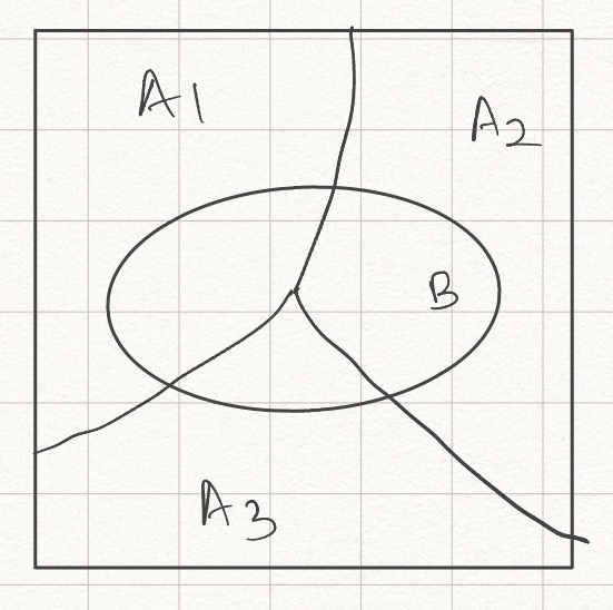
Fig. 1. Partitioned Sample Space.
Let the sample space be partitioned into three events \(A_1\), \(A_2\) and \(A_3\) as shown in Fig 1. Now there is another event \(B\). We know the probability of event \(B\) occuring given event \(A_i\) has occured. What is the probability of event \(B\) occuring. That is given by the total probaility theorem:
\[P(B) = P(A_1)P(B \mid A_1) + P(A_2)P(B \mid A_2) + P(A_3)P(B \mid A_3)\]Bayes’ rule
Let the sample space be partitioned into three events \(A_1\), \(A_2\) and \(A_3\) as shown in Fig 1. Now there is another event \(B\). Given that \(B\) has happened, we want to know the probability of event \(A_i\) happening. This is given by Bayes rule
We know the individual probabilities of each \(P(A_i)\). We also know the probability \(P(B \mid A_i)\) for each \(i\). Based on these knowledge, we can find \(P(A_i \mid B)\) as:
\[\begin{align} P(A_i \mid B) &= \frac{P(A_i \cap B)}{P(B)} \\ &= \frac{P(A_i)P(B \mid A_i)}{P(B)} \\ &= \frac{P(A_i)P(B \mid A_i)}{\sum_j P(A_j)P(B \mid A_i)} \end{align}\]Bayes’ rule tells us that given an effect \(B\), what are the chances of the cause being \(A_i\).
Independence
Suppose we are tossing a coin. We know that the probability of getting a head is \(P\) and the probability of getting a tail is \((1-P)\). Suppose we toss the coin once. Then the probability of getting a head will be \(P\). If we toss the coin a second time, the probability of getting a head will still be \(P\). It won’t change nomatter what was the outcome of the first toss. This is called even. The two tosses are independent events.
Mathematically, we can write it as
\[P(B \mid A) = P(B)\]if the occurance of \(A\) provides no information on the occurance of \(B\).
In case of two independent events,
\[P(A \cap B) = P(A)P(B \mid A) = P(A)P(B)\]Thus two events \(A\) and \(B\) are said to be independent if
\[P(A \cap B) = P(A)P(B)\]NOTE: Disjoint events doesn’t mean they are independent. Ex: In a sample space, suppose there are two disjoint events \(A\) and \(B\). Then if we know that event \(A\) has occured, we can say that event \(B\) has not occured.
Conditional Independence
Given an event \(C\) has occured, two events \(A\) and \(B\) are said to be conditionally independent, if
\[P(A \cap B \mid C) = P(A \mid C) P(B \mid C)\]